Python: Geographic Object-Based Image Analysis (GeOBIA) – Part 1: Image Segmentation

This tutorial will walk you through segmenting and classifying high resolution imagery using Python. Part 1 of this tutorial teaches how to segment images with Python. After you have completed Part 1, Part 2 will teach how to use machine learning methods to classify segments into land cover types with Python.

YouTube videos give step-by-step instructions throughout the tutorials. This tutorial picks up after the Python interpreter is set up and all the necessary packages have been downloaded. To view the entire process from start to finish, including downloading the images shown in this post, and setting up the Python interpreter, follow the video tutorials in the YouTube playlist.

The first step is to read data from the NAIP image into python using gdal and numpy. This is done by creating a gdal Dataset with gdal.Open(), then reading data from each of the four bands in the NAIP image (red, green, blue, and near-infrared). The code and video below give the specifics of the process.

import numpy as np
import gdal
from skimage import exposure
from skimage.segmentation import quickshift
import time

naip_fn = 'C:/temp/naip/m_4211161_se_12_1_20160624.tif'

driverTiff = gdal.GetDriverByName('GTiff')
naip_ds = gdal.Open(naip_fn)
nbands = naip_ds.RasterCount
band_data = []
print('bands', naip_ds.RasterCount, 'rows', naip_ds.RasterYSize, 'columns',
      naip_ds.RasterXSize)
for i in range(1, nbands+1):
    band = naip_ds.GetRasterBand(i).ReadAsArray()
    band_data.append(band)
band_data = np.dstack(band_data)

Once the image data have been read into a numpy array the image is be segmented. In this tutorial, we use the skimage (scikit-image) library to do the segmentation. This library implements a number of segmentation algorithms including quickshift and slick, which are what we use in this tutorial. First we rescale the image values so they are between zero and one, then we do the segmentation. Documentation for segmentation algorithms is available at https://scikit-image.org/docs/dev/api/skimage.segmentation.html

# scale image values from 0.0 - 1.0
img = exposure.rescale_intensity(band_data)

# do segmentation multiple options with quickshift and slic
seg_start = time.time()
# segments = quickshift(img, convert2lab=False)
# segments = quickshift(img, ratio=0.8, convert2lab=False)
# segments = quickshift(img, ratio=0.99, max_dist=5, convert2lab=False)
# segments = slic(img, n_segments=100000, compactness=0.1)
# segments = slic(img, n_segments=500000, compactness=0.01)
segments = slic(img, n_segments=500000, compactness=0.1)
print('segments complete', time.time() - seg_start)

# save segments to raster
segments_fn = 'C:/temp/naip/segments.tif'
segments_ds = driverTiff.Create(segments_fn, naip_ds.RasterXSize, naip_ds.RasterYSize,
                                1, gdal.GDT_Float32)
segments_ds.SetGeoTransform(naip_ds.GetGeoTransform())
segments_ds.SetProjection(naip_ds.GetProjectionRef())
segments_ds.GetRasterBand(1).WriteArray(segments)
segments_ds = None

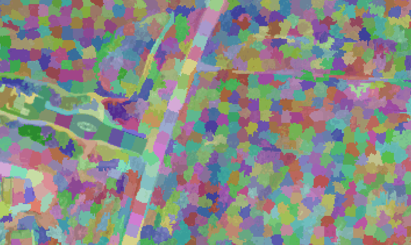
Image segmentation

Images below show the segments generated from different parameter combinations of the quickshift and SLIC algorithms, with the code used to create each segmentation. The segments are 50% transparent over the NAIP image to show how the segments represent image features. Only a portion of the NAIP image is used for comparisons.

Quickshift segmentation

The segments below were generated with the quickshift defaults. As you can see, these segments were too large to accurately represent the roads in the NAIP image. The initial segmentation did not match image objects very well so I hanged the algorithm parameters so get a more appropriate segmentation result.

segments = quickshift(img, convert2lab=False)

The ratio parameter ranges from 0-1 with values close to zero creating segments based on distance (more regularly shaped) and values close to one creating segments based on color (more irregularly shaped). As you can see from the image below, changing the ratio parameter did not create segments that were obviously different from the default parameter.

segments = quickshift(img, ratio=0.8, convert2lab=False)

The max_dist parameter controls the relative output size of the segments. Below, I decreased the max_dist parameter from the default value of 10 to create more, smaller segments. As a result, you can see these segments are smaller and do a better job of capturing features in the image.

segments = quickshift(img, ratio=0.99, max_dist=5, convert2lab=False)

SLIC segmentation

The SLIC segmentation is largely controlled by the approximate number of segments (n_segments) and shape (compactness) of the segments. Therefore, I started with 100,000 segments because the quickshift algorithm was producing 50,000-75,000 segments and not capturing enough detail. As you can see from the image below, slic seems to do a better job at capturing features in this image than quickshift.

segments = slic(img, n_segments=100000, compactness=0.1)

Increasing the number of segments and decreasing the compactness resulted in very elongated segments, and didn’t seem to match the image features very well.

segments = slic(img, n_segments=500000, compactness=0.01)

This is the best segmentation (below) I was able to create (with the limited runs I performed). As you can see, a segmentation that represents image features is very important to creating accurate classifications.

segments = slic(img, n_segments=500000, compactness=0.1)

Spectral Properties of Segments

Now we need to describe each segment based on it’s spectral properties because the spectral properties are the variables that will classify each segment as a land cover type.

First of all, write a function that, given an array of pixel values, will calculate the min, max, mean, variance, skewness, and kurtosis for each band. The code below takes all the pixels in a segment and calculates statistics for each band, saving them in the features variable, which is returned. Next, get the pixel data and save the returned features. I describe this process below.

def segment_features(segment_pixels):
    features = []
    npixels, nbands = segment_pixels.shape
    for b in range(nbands):
        stats = scipy.stats.describe(segment_pixels[:, b])
        band_stats = list(stats.minmax) + list(stats)[2:]
        if npixels == 1:
            # in this case the variance = nan, change it 0.0
            band_stats[3] = 0.0
        features += band_stats
    return features

In object-based image analysis each segment represents an object. Objects represent buildings, roads, trees, fields or pieces of those features, depending on how the segmentation is done. The code below gets a list of the segment ID numbers. Then sets up a list for the statistics describing each object (i.e. segment ID) returned from the segment_features function (above). The pixels for each segment are identified and passed to segment_features, which returns the statistics describing the spectral properties of the segment/object. Statistics are saved to the objects list and the object_id is stored in a separate list. Note: depending on how many segments are in your image, this code could take several hours to run. For the image used in this tutorial it took my Dell XPS with an Intlel i7 8565U processor about 6 hours. This code block could be parallelized, and I may show how to do that in a future post.

segment_ids = np.unique(segments)
objects = []
object_ids = []
for id in segment_ids:
    segment_pixels = img[segments == id]
    object_features = segment_features(segment_pixels)
    objects.append(object_features)
    object_ids.append(id)

outro to post here