Supervised Image Classification with QGIS
Image classification techniques are at the heart of modern remote sensing. Image classification is a method of extracting usable information from images. Without classification, images are just a collection of numbers that represent colors and it’s very difficult to obtain any quantifiable information about a landscape from data like that.
With remote sensing techniques, we can extract information from images to analyze landscapes and how they change over time. One of the most-used remote sensing techniques is supervised image classification. With supervised classification, a user identifies areas of the image that represent land cover classes of interest. These areas are marked and used to train a computer algorithm to identify those same land cover classes throughout the entire image and in other images. There are many software companies that have expensive products designed to help you accomplish these tasks. But you can do this for free with QGIS.
This tutorial will walk you through creating a land cover classification for a Landsat 9 image. Though I’ll be using Landsat 9 in this tutorial, you can apply this same workflow to classify images from any other source. Let’s get started!
Install the Semi-automatic Classification Plugin
There is a lot of math and data management required to perform any kind of classification with satellite or aerial imagery. The Semi-automatic Classification Plugin (SCP for short) for QGIS will take care of all this behind the scenes. SCP is free and can be installed right in QGIS.
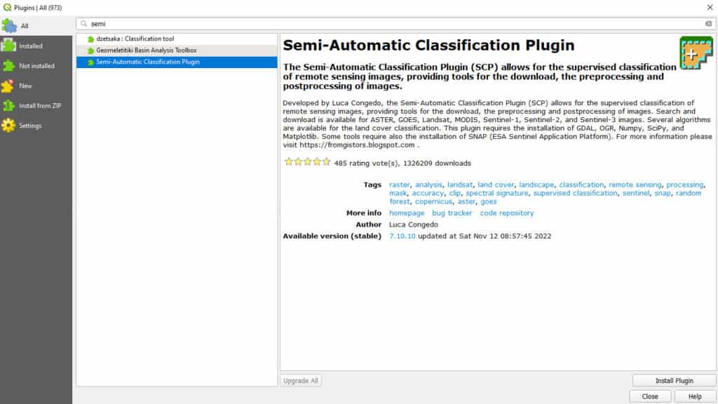
To install SCP, navigate to Plugins > Manage and Install Plugins on the QGIS Main Menu. This will open up the QGIS Plugin Manager window. Make sure you have selected ‘All’ on the left side. Now start searching for “Semi-automatic Classification Plugin”. You should see it appear. Click on the plugin name. Then click the ‘Install’ button and wait for the installation to complete.
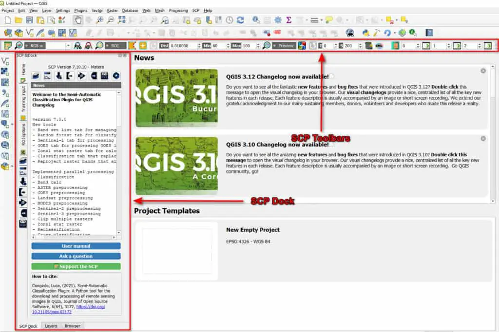
Once you have SCP installed you should see a new panel (SCP Dock) and two new toolbars (SCP Working Toolbar and SCP Editing Toolbar) have been added to your QGIS interface (see image below). If these features have not been added you can go to View > Panels, or View > Toolbars to add them. You will also see a new ‘SCP’ option on the QGIS Main Menu.
Now we’re ready to get started with some classification!
Open Landsat Data
For this tutorial, I’m going to be using Landsat 9 Analysis Ready Data (ARD). This same dataset is available to students of my Remote Sensing with QGIS course (along with many other datasets). The Landsat 9 ARD data can also be downloaded for free.
You can also use any other satellite or aerial imagery that you have available. Just note that some of the steps in this tutorial may be slightly different for you if you are using a different dataset.
Add the .TIF files for Landsat 9 bands 1-7 into the QGIS interface. You will need to have these files open in QGIS in order to create a band set in the next step.
Create a Band Set with SCP
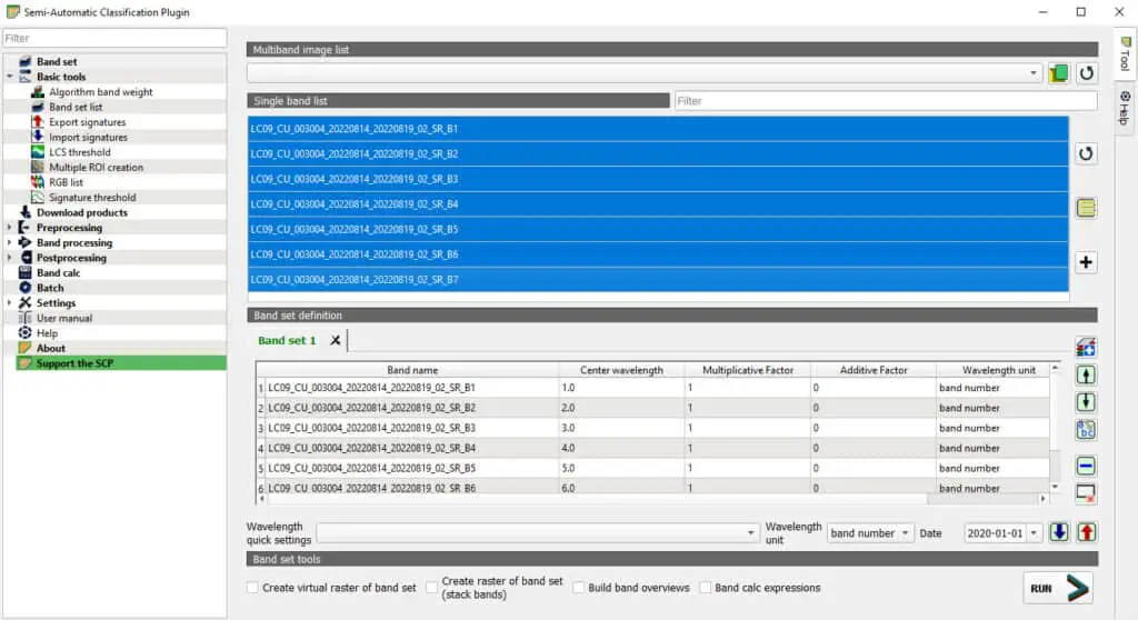
Open the SCP Band Set window with SCP > Band Set from the Main Menu. Now click the refresh button ![]() to bring in the bands you just loaded into QGIS. Initially, the bands will appear in the ‘Single band list’ portion of the window. Select all the bands you want to use for the classification (you can hold CTRL to select multiple bands) and click the add button
to bring in the bands you just loaded into QGIS. Initially, the bands will appear in the ‘Single band list’ portion of the window. Select all the bands you want to use for the classification (you can hold CTRL to select multiple bands) and click the add button ![]() to add the bands to the band set. Your screen should look similar to the image below.
to add the bands to the band set. Your screen should look similar to the image below.
Defining Regions of Interest
Once the band set is ready we can start defining regions of interest, or ROIs. Defining ROIs is the supervised part of supervised classification. In this step, we’ll draw polygons to represent the different land cover classes that we want to represent. Then we’ll use SCP to do the math that uses information from our sample ROIs to train an algorithm that will predict land cover for the rest of the image.
Create a Training Input File
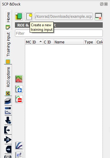
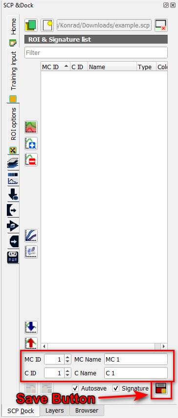
Before we start defining ROIs, we need to create a file to save the ROI information. Go to the SCP Dock panel and click on the ‘Training Input’ tab (on the left side, see the image below). Now click the button to create a new training input ![]() . Choose a location for your file and give it a name. Creating the training input file will also create a new vector layer where you will be able to see the ROIs you create. This layer will be named the same as your training input file and will be added to the table of contents (Layers panel) automatically.
. Choose a location for your file and give it a name. Creating the training input file will also create a new vector layer where you will be able to see the ROIs you create. This layer will be named the same as your training input file and will be added to the table of contents (Layers panel) automatically.
Display a True Color Image
Unless you’ve made some changes on your own then all of your imagery bands are still being displayed in grayscale. This makes it difficult to see the land cover classes we want to identify. Let’s use SCP to make a true-color image.
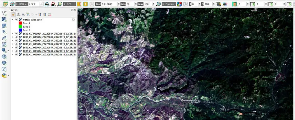
On the SCP toolbar look for a box with RGB= next to it. In the box enter 4-3-2 and push Enter/Return (see image below). This will create a new Virtual Band Set in your QGIS Table of Contents (i.e., Layers panel, you may need to switch over to the Layers panel to see it). Reorder your layers so the new virtual layer is on top and you’ll have a color image. Note that 4-3-2 correspond to the red, green, and blue bands for Landsat 9. If you are using a different imagery source you’ll have to adjust the band numbers accordingly.
Create ROIs
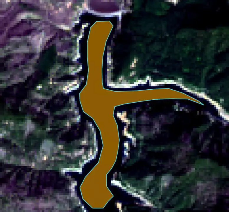
We now have everything set up to start creating ROIs. Make sure you have your SCP Dock and SCP toolbars available and visible. To create an ROI click on the Create ROI button ![]() on the SCP toolbar. Now left-click to place vertices of a polygon that outlines a region of interest corresponding to a single land cover type. When you’re ready to finish the polygon, right-click to complete. You can see the ROI I’ve create to represent a portion of a lake in the image below.
on the SCP toolbar. Now left-click to place vertices of a polygon that outlines a region of interest corresponding to a single land cover type. When you’re ready to finish the polygon, right-click to complete. You can see the ROI I’ve create to represent a portion of a lake in the image below.
Once your ROI polygon is complete go back to the SCP Dock. At the bottom of the panel, you will see four input boxes labeled with ‘MC ID’, ‘MC Name’, ‘C ID’, and ‘C Name’. This is where you will specify the names and identifiers for the Master Class (MC) and Class (C). For my lake ROI I’m going to keep the MC ID as 1 and change the MC Name to ‘Water’. I’ll also keep the C ID as 1 and change the C Name to ‘Lake’. Once you have set these variables click the save to training input button ![]() to save the spectral signature inside the ROI polygon to the training data file.
to save the spectral signature inside the ROI polygon to the training data file.
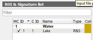
It will take just a minute to save the spectral data associated with the ROI. Once it is saved you will see the ROI added to the ‘ROI & Signature list’.
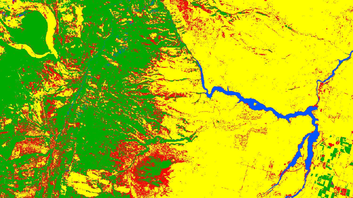
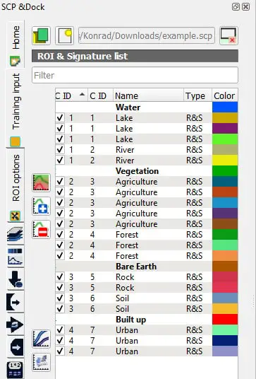
Create more ROIs to characterize the land cover classes of your landscape. For this example, I have created four Macro Classes: water, vegetation, bare earth, and built-up. I’ll use these classes for my final classification. You’ll want to do a good job of selecting ROIs that distinguish differences between the land cover classes you’re interested in.
You can make changes to ROIs (including the color) by right-clicking on a Macro Class or Class in the list and adjusting the available settings. You will find additional information in the ‘Properties’ option.
Note: SCP contains methods to automatically create ROIs (instead of manually clicking for each vertex). There’s not room to cover those methods in this tutorial, but they are covered in my Remote Sensing with QGIS course.
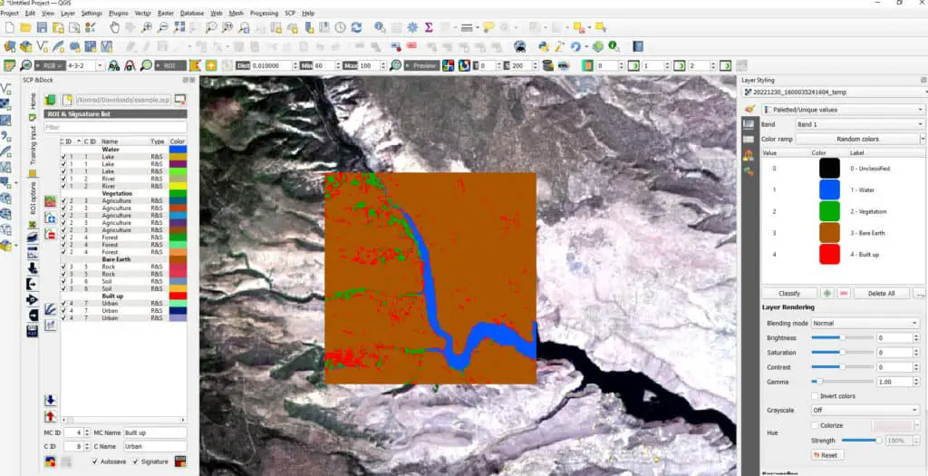
Generate a Classification Preview
With SCP we can generate a classification preview to have a preliminary assessment of our classification for a portion of the study area before we perform the full classification. This gives us a chance to determine if we might need to adjust our ROIs, or add more ROIs, before doing a classification of the full image.
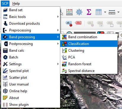
Before generating a preview, check the SCP classification settings. Go to SCP > Band Processing > Classification. Here you can adjust the classification algorithm and at which class level (Macro Class or Class) the classification will occur. My settings are to classify the Macro Class using the Minimum Distance algorithm with the threshold set to 0.0. You can play around with these settings to see how it changes the resulting classification.
To generate the preview, click the ‘Activate classification preview pointer’ button ![]() on the toolbar. Now click a location on the map where you want the preview to generate. The
on the toolbar. Now click a location on the map where you want the preview to generate. The S option on the toolbar will adjust the size of the preview area. A new, temporary layer will be added to the Layers panel. This layer contains the classification preview. It will display automatically.
You can adjust the color or classification settings and click the ‘Refresh’ button, next to the preview generation button, to regenerate the preview.
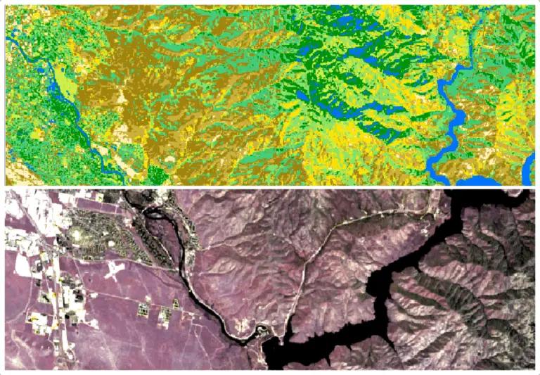
Perform the Full Classification
Once you’re happy with the classification preview, you can apply the classification to the entire image. To do this go back to SCP > Band processing > Classification. Choose the settings you wish to apply. Then click Run. You will be prompted to specify an output file for the classification. Then the classification will execute. It will take a few minutes to complete. Once the classification is completed, the classified image will automatically be added to QGIS where you can view it.
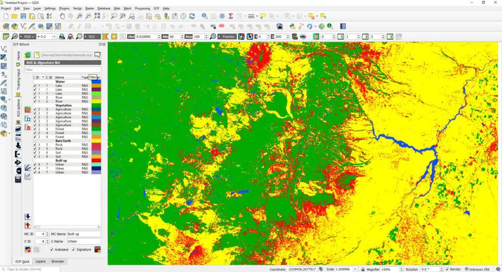
That’s it! You’ve successfully performed supervised image classification in QGIS!
Conclusion
If you’ve made it this far, congratulations! I hope you were able to follow along and perform the supervised classification. Even though we covered a lot of ground in this tutorial, we barely touched the surface of remote sensing with QGIS. If this article piqued your interest and you’re looking for a more in-depth experience with QGIS remote sensing, I suggest you check out my full remote sensing course. If you’re looking for more free tutorials, you might find the links below useful.