Unsupervised Land Cover Classification with Python

Aerial imagery is used for purposes ranging from military actions to checking out the backyard of a house you might buy. Our human brains can easily identify features in these photographs, but it’s not as simple for computers. Automated analysis of aerial imagery requires classification of each pixel into a land cover type. In other words, we must train a computer to know what it’s looking at, so it can figure out what to look for.

There are two primary classification methods. Supervised and unsupervised. Supervised classification uses observed data to teach an algorithm which combinations of red, green, and blue light (pixel values in an image) represent grass, trees, dirt, pavement, etc. Unsupervised classification assigns pixels to groups based on each pixel’s similarity to other pixels (no truth, or observed, data are required).

I previously described how to implement a sophisticated, object-based algorithm for supervised image analysis. This article describes simple implementation of the K-Means algorithm for unsupervised image classification. Because unsupervised classification does not require observational data (which are time consuming, and expensive, to collect) it can be applied anywhere.

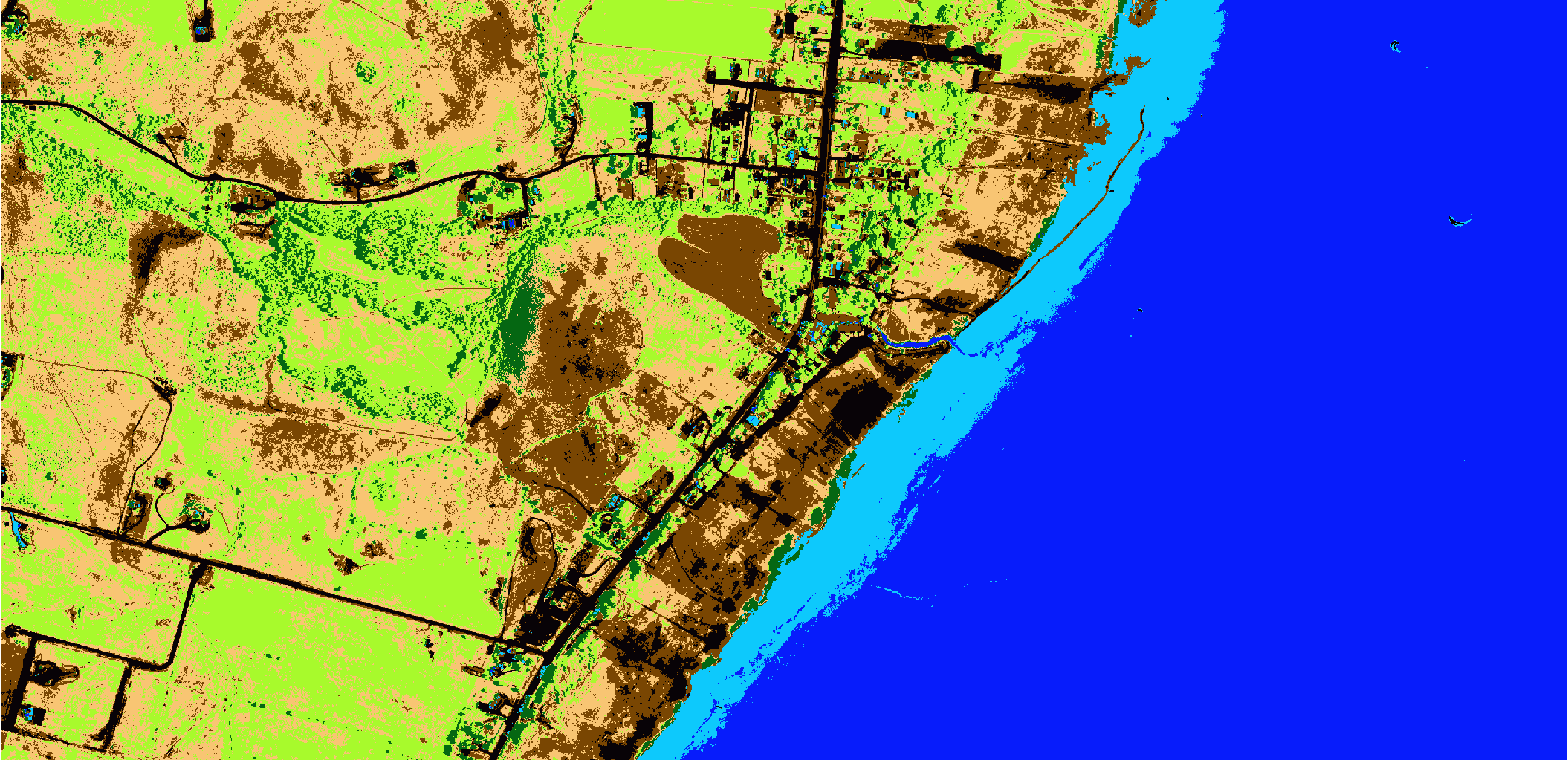
We will use a portion of an image from the National Agricultural Imagery Project (NAIP, shown below). A gist containing all the code is presented at the end of the article.

Getting Started

Only three Python modules are required for this analysis. scikit-learn (or sklearn), gdal, and numpy.

Import the modules and load the image with gdal. Query the number of bands in the image (gdal dataset) with RasterCount. Depending on the sensor used to collect your image you could have between 3 and 500 (for hyperspectral imagery) bands. NAIP has 4 bands that quantify the reflectance red, green, blue, and near-infrared light.

Also, create an empty numpy array to hold data from each image band. We will flatten the data to work better with the sklearn k-means algorithm. The empty array needs as many rows as the product of rows and columns in the image, and as many columns as raster bands.

from sklearn.cluster import KMeans
import gdal
import numpy as np

naip_fn = 'path/to/image.tif'
driverTiff = gdal.GetDriverByName('GTiff')
naip_ds = gdal.Open(naip_fn)
nbands = naip_ds.RasterCount
data = np.empty((naip_ds.RasterXSize*naip_ds.RasterYSize, nbands))

Read the data for each raster band. Convert each 2D raster band array to a 1D array with numpy.flatten(). Then add each array to the data array. Now all the band data are in a single array.

for i in range(1, nbands+1):
    band = naip_ds.GetRasterBand(i).ReadAsArray()
    data[:, i-1] = band.flatten()

K-means Classification

We can implement the k-means algorithm in three lines of code. First set up the KMeans object with the number of clusters (classes) you want to group the data into. Generally, you will test this with different numbers of clusters to find optimal cluster count (number of clusters that best describes the data without over-fitting). We won’t cover that in this article, just how to do the classification. After the object is set up fit the clusters to the image data. Finally, use the fitted classification to predict classes for the same data.

km = KMeans(n_clusters=7)
km.fit(data)
km.predict(data)

Save the Results

Retrieve the classes from the k-means classification with labels_. This returns the class number for each row of the input data. Reshape the labels to match the dimensions of the NAIP image.

out_dat = km.labels_.reshape((naip_ds.RasterYSize, naip_ds.RasterXSize))

Finally, use gdal to save the result array as a raster.

clfds = driverTiff.Create('path/to/classified.tif', naip_ds.RasterXSize, naip_ds.RasterYSize, 1, gdal.GDT_Float32)
clfds.SetGeoTransform(naip_ds.GetGeoTransform())
clfds.SetProjection(naip_ds.GetProjection())
clfds.GetRasterBand(1).SetNoDataValue(-9999.0)
clfds.GetRasterBand(1).WriteArray(out_dat)
clfds = None

Conclusion

It is quite simple to implement an unsupervised classification algorithm for any image. There is one major drawback to unsupervised classification results that you should always be aware of. The classes created with unsupervised methods do not necessarily correspond to actual features in the real world. The classes were created by grouping pixels with similar values for all four bands. It is possible that the roof of a house could have similar spectral properties as water, so rooftops and water might get confused. Caution is imperative when interpreting unsupervised results.