Up next in 10

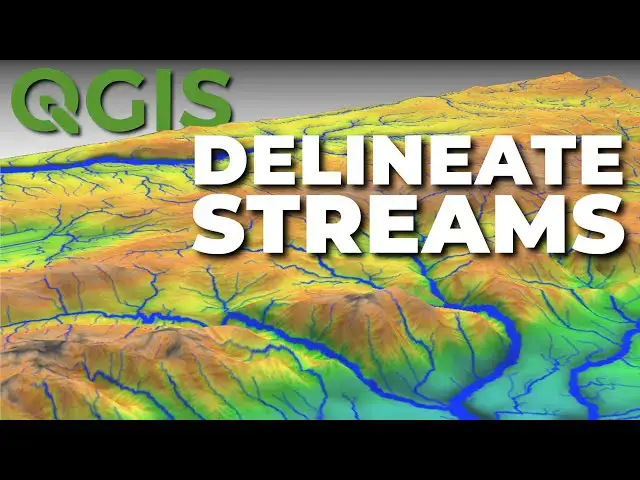
Learn how to delineate streams from a DEM in QGIS using the GRASS tools.
Check out my website for more: https://opensourceoptions.com
Show More Show Less View Video Transcript
0:01
Welcome to Open Source Options. In this
0:04
demonstration, I'm going to show you how
0:05
we can take a digital elevation model
0:07
like this and extract vectorzed
0:11
streamlines from it. Uh, and we have a
0:14
few steps to go through to do that.
0:16
Before we get started on this, I just
0:18
want to remind you that my first course,
0:20
GIS Foundation, will soon be available
0:23
on opensource options.com. You can go to
0:26
opensource options.com and sign up for
0:28
emails to be notified when that course
0:30
is available. Following that course,
0:33
additional courses are going to start
0:34
coming out. So, thanks for supporting me
0:36
there. And I should mention that all
0:38
these courses are going to be completely
0:41
free. Okay, let's get started with our
0:44
demo for today on delineating watersheds
0:48
and streamlines. Now, you'll notice here
0:50
I have a digital elevation model loaded.
0:52
I downloaded this from the USGS ladder
0:56
explorer and I used a digital elevation
0:59
model of 10 meters or 1/3 arcsec. Uh I
1:03
did this so we don't have super high
1:04
resolution because I want to make sure
1:06
the computation goes quickly uh instead
1:08
of being slow.
1:11
Now this was from a much larger DEM to
1:14
start. Here's the original DEM.
1:17
And I clipped out a small area. You can
1:20
see it here. And this is just for
1:22
computational purposes so that we don't
1:25
have large data sets working with and
1:27
the computations can occur quickly. And
1:29
then this was in a geographic coordinate
1:32
system. So I projected it into UTM so
1:35
that we could work in linear units if we
1:37
need to do any calculations. Okay, very
1:40
simple to do. And I have videos on how
1:42
to download the data uh and on flipping
1:46
that you can also watch for more
1:48
information there. All right, now let's
1:49
get into this. We're going to use the
1:52
Grass GIS tools for this tutorial. So,
1:56
you need to have QGIS installed with
1:58
Grass. I also have a video on how to do
2:00
that. This it shows my preferred method
2:02
for installing and updating QGIS. And if
2:05
you follow that, it's really easy to add
2:07
or update any aspects of QGIS.
2:11
The first tool we'll use in grass is the
2:15
R doilder.
2:19
And direction. this one here. You can
2:21
search for this in this in the locate
2:23
bar if you need to do that. I'm going to
2:26
open this tool up. This tool does two
2:28
things. It calculates a depressionless
2:31
DEM and it calculates flow directions.
2:35
All we need from this is the
2:38
depressionless DEM. Now, we need to make
2:40
sure that we're working from our
2:42
projected DEM, which is this one here.
2:45
Uh we can leave the defaults.
2:48
I'm going to come down and I'm not even
2:50
going to save the flow directions or the
2:52
problem areas. I'll turn those off, but
2:54
I'll save this depressionless DEM to a
2:57
file
2:58
and I'm going to save that here. I'm
3:00
going to overwrite a file I created
3:01
earlier. I'm going to overwrite this
3:02
field file and we'll click save and I'll
3:05
say yes. And I will run this.
3:10
Okay. And we can see we had some errors.
3:12
Those are not big deals. It's just a
3:13
color table error. It's not going to
3:15
cause any issues. and we get this output
3:17
which is has a default style like this
3:20
called field. Now I'm going to remove
3:22
these two elevation models that we're
3:24
not using just so we can simplify our
3:27
layers here. Now I want to show you what
3:29
this field layer looks like uh and what
3:32
actually happened here. So I'm going to
3:34
do that by using a raster calculator
3:37
calculation. I'm going to take this
3:40
filled elevation model and I'm going to
3:42
subtract from it our original. And I'm
3:45
going to create an on the-fly raster and
3:47
say okay.
3:49
Going to drag this up to the top. You'll
3:52
notice it's mostly black. The values
3:54
range from zero to positive4. Let's go
3:57
style this so we can see uh what it
4:00
looks like. Let's change this to single
4:02
band pseudo color. This red's palette is
4:04
just fine. any pallet will probably work
4:07
uh suitably for this. And now I'm going
4:09
to just go to the zero value here and
4:12
I'm going to double click on it and come
4:15
down and change the opacity to zero. I'm
4:17
going to turn off this well going to
4:20
drag this up so we can have a little
4:22
more contrast. I'm going to zoom in on
4:23
some of these areas.
4:26
Now go to my value plug value tool
4:28
plugin. You can see we have our original
4:30
DEM and our field DEM. When I hover over
4:33
these, you can see that we have some
4:35
differing values. For example, here the
4:38
difference is about a half meter between
4:40
the original and the field with the
4:42
field being a halfmeter higher in
4:44
elevation in these pixels. And we can
4:47
see some other locations where this
4:49
happens like along here in what appears
4:52
to be maybe the stream channel.
4:55
Now, what's happening here is the way
4:57
this algorithm works, the algorithms
4:58
we'll use work, they're going to route
5:00
flow downhill. when we get to these
5:03
areas, these pixels here, every
5:06
direction from these pixels is uphill.
5:07
So, there's nowhere to route flow. And
5:09
when that happens, the algorithm will
5:11
stall out. Um, it won't cause any errors
5:14
necessarily, but our stream lines won't
5:16
be connected because there's nowhere for
5:17
water to flow from these pixels. So, the
5:20
filling we just did filled those pixels
5:22
and it added um it increased their
5:24
values so that water can flow through
5:26
them and we get an idea of where our
5:28
stream will actually go. So that was
5:30
that was our first step. We can now
5:32
remove this layer. We don't actually
5:34
need to have this raster calculator. We
5:36
just need this field elevation model.
5:38
And this will be our base DEM that we
5:40
use for the inputs to the other tools
5:43
that we are calculating.
5:46
Now that we have our field DEM
5:48
calculated, we can go through and
5:49
calculate what is called the flow
5:50
accumulation.
5:52
And the flow accumulation will
5:53
accumulate that water downstream. So we
5:56
can see the direction the water flows
5:57
across the landscape. Let's go back to
5:59
the processing toolbox. We're going to
6:01
be using our grass tools again. So,
6:03
we're going to find R.watershed, which
6:05
will calculate this and other metrics.
6:08
So, we go to R.h.
6:11
Open this up. There are a few things
6:14
that we need to set. Um, the first we
6:17
need to make sure this is set to our
6:19
filled dem.
6:21
Next, we need to make to set this
6:23
minimum size of exterior watershed
6:26
basin. If this is not set, you will
6:28
probably get some errors. For this DE,
6:30
I'm going to set it to 100. The
6:33
documentation states that if you set
6:34
this value too low, it could lead to
6:37
errors. So, if you experience errors in
6:39
this calculation, you might want to
6:41
increase that value up to 500 or more.
6:47
Now, we need to set a couple of other
6:48
things here. We're going to enable
6:50
single flow direction, which is a very
6:52
simple way to calculate these flow
6:54
directions. Um we can use the default of
6:56
multiple flow direction. Uh but this is
6:58
the D8 version which you might be most
7:00
familiar with where water from one cell
7:03
uh flows only to one cell instead of to
7:06
multiple cells. And you can look up D8
7:09
and multiple flow direction MFD
7:10
differences to get a better idea of of
7:13
how those differ. And now uh we also
7:16
want to use positive flow accumulation
7:19
even for likely underestimates. This
7:21
will just give us smooth streamlines and
7:23
not have negative values in those
7:24
streamlines which can happen if we uh if
7:28
we don't check this box. So those are
7:31
the three parameters to set. Check these
7:32
two boxes and change
7:35
um your minimum size of exterior
7:37
watershed basin.
7:39
Now let's go look at the outputs. We
7:42
have a number of outputs. The only one
7:45
we actually need to save is the number
7:47
of cells that drain through each cell.
7:49
And we're going to save this to a file.
7:52
I'm going to call this accumulation. I'm
7:54
going to click save. I'll replace that
7:56
file that I've used in testing. And now
7:59
I'm going to turn off all these other uh
8:02
options. We have drainage direction,
8:05
which we're not going to need. Flow
8:06
direction. Uh we have watershed basins.
8:11
Uh we have
8:13
slope. We have topographic index. We
8:16
have stream power index. a lot of
8:19
different files, but we only need the
8:20
flow accumulation to calculate or to
8:23
determine where our streams run. I'm
8:25
going to run this tool now. Let's take
8:27
just a second to process.
8:30
And there we go. There are no errors.
8:33
Let me pull this flow accumulation to
8:34
the top here. And now you can see the
8:38
way that Grass has styled this. We have
8:42
the higher values are showing as black
8:44
and the lower values are showing as
8:46
yellow. So if we go to our value tool,
8:48
we can get an idea for what these values
8:50
are. Look at this accumulation layer
8:52
here. So in the yellow, you can see we
8:53
have very low values. In the green,
8:55
those values start to move up. And as we
8:57
get into blues, we're starting to get to
8:59
larger values. Um in the hundreds, we're
9:03
starting to see these stream channels
9:04
appearing. And as we get to black, we
9:06
even have much higher values in the
9:08
thousands. Now, we can use the value
9:10
tool to kind of get an idea of how to
9:12
delineate these streams. So the streams
9:15
I want to delineate are this main stream
9:17
that comes here. This one is called
9:18
Spawn Creek is a tributary to Temple
9:21
Fork, which we don't have all of the DEM
9:23
for Temple Fork. So we're not going to
9:24
be able to delineate the whole stream.
9:26
You can see Temple Fork runs basically
9:28
through here.
9:30
Let's go and see what this values the
9:32
accumulation values of these streams
9:33
are. You can see that we're above 10,000
9:36
up in these headwaters. These are
9:38
probably even before the stream starts.
9:40
We're above 5,000 in a lot of these
9:42
areas. 10,000 9,000. We come down a
9:46
little ways to where the tribute Freddy
9:47
comes in, we have values of just over
9:50
19,000.
9:51
If we come down and look at Temple Fork
9:54
and these upper leeches here, you can
9:55
see we have values of 5,000. As we come
9:58
down into this location here, you can
10:01
see we have values of around 19,000
10:03
there.
10:06
We have some streams coming off the
10:07
backside here. We can take a look and
10:09
see what these accumulation values are.
10:11
And you can see that we're about 22,000
10:14
just over 22,000 for some of those
10:16
stream segments. And let's look at some
10:18
of these larger tributaries of Spawn
10:19
Creek. You can see that this tributary
10:22
here has values of about 7,000.
10:25
This one here
10:27
of about 10,000
10:30
and this one here
10:33
of about 10,000. So to exclude these
10:36
larger tree headers, we're going to need
10:37
to have a threshold above 10,000.
10:41
Another way to look at this is we can
10:42
use a raster calculator
10:45
to visualize this a little more cleanly.
10:47
So we can come to raster raster
10:49
calculator and we can calculate where
10:52
our accumulation is greater than a
10:54
threshold. So let's say we want let's
10:56
look at 10,000 for example 10,000. We'll
10:59
create an on the-fly raster and we'll
11:02
click okay.
11:04
accumulation is here. So, we're going to
11:05
slide that up and you can see that we're
11:08
showing as a value of one everywhere
11:11
that our flow accumulation is greater
11:13
than 10,000 and we can see how those
11:15
streams will map out. Let's remove this
11:18
and try a different threshold of say
11:19
20,000.
11:22
So, let's go back to raster raster
11:24
calculator accumulation
11:27
uh is greater than 20,000
11:30
and create on the fly raster again.
11:32
Click okay. And there you can see that
11:34
we're capturing our main stream of spawn
11:37
creek which is different temple for it's
11:39
not fully included in our raster. And we
11:41
have a minimal stream segment over here
11:43
for different a different uh stream that
11:46
comes off of that side. Okay. So I think
11:49
I'll use a first 20,000. You'll see
11:50
where this plays in later. So I'll
11:53
remove this layer.
11:55
Now the next tool we want to use is R
11:59
stream extract from grass. So
12:03
R.stream.extract.
12:06
And here we're going to input our field
12:09
elevation. We're going to input our flow
12:13
accumulation.
12:15
And now we can set a minimum flow
12:17
accumulation for stream. So we can set
12:19
this to 20,000.
12:25
And we can we can adjust stream
12:28
segments. They need to be at least 100
12:30
cells long or it won't include them. You
12:34
can leave that at zero if you like to
12:35
have you might have some short stream
12:37
segments which is okay.
12:41
We can leave all of these as the
12:43
defaults.
12:45
RV.out.gr
12:47
output type
12:49
to use line. So give us a line out for
12:51
our streams.
12:54
And now we can save our layers. So this
12:57
will give us unique stream ids as a
12:59
raster. So let's save this to a file. So
13:03
let's call this stream ID.
13:09
This will give us unique stream ids as a
13:12
vector.
13:16
So let's save this to file. We'll just
13:18
call this
13:19
streams. We'll save it as a go package
13:24
and we don't need to save the flow
13:25
direction. So we'll just uncheck that
13:27
and leave it as temporary. Let's go
13:29
ahead and click run.
13:35
Okay, so we don't see any errors. We
13:37
just see a color table error which
13:39
should not be a problem. We can close
13:41
this. You can see that our streams,
13:43
these two layers are now added. Let's
13:45
turn off our accumulation. Let's turn
13:48
off uh these layers.
13:52
We'll leave that one on because it's got
13:53
some good contrast. So now we can zoom
13:56
in and we can see that by limiting the
13:58
the threshold to streams greater than
14:01
100 pixels, we have a single stream that
14:03
occurs here. And let me just show you
14:06
what this looks like. So if we take this
14:07
off, you can see this occurs. This has
14:09
pixel values. This is a raster. And we
14:12
can go to our value tool and we can see
14:14
that it just has a value of one.
14:17
Let's go back and rerun this again with
14:20
a different um minimum length so that we
14:23
can see what it looks like with multiple
14:24
streams. So if we go back to um
14:28
processing and history, we can go to
14:31
r.stream.extract and pull up our exact
14:35
parameters.
14:37
We can set this to zero
14:41
and we can come down and change our file
14:44
names to stream ID2 and streams 2. And
14:47
we can click run to create these layers
14:49
again.
14:51
Let's go ahead and close that. Oh, I
14:53
left the flow direction on that time so
14:55
you can see our flow direction values,
14:57
but let's just remove those.
15:01
Okay. Now I'll turn off these
15:05
and we'll turn off this. And you can see
15:07
here we now have four stream segments.
15:10
So if I hover over these, you can see we
15:12
have a value of four, a value of one, a
15:16
value of three, and over here this short
15:19
segment gives us a value of two.
15:25
Oops, widen that out on accident. And if
15:29
we now turn these streams on, we can see
15:32
that purple line. Uh we can open this
15:35
attribute table up and you can see that
15:38
we have a feature ID. Um this category
15:43
or cat, we have a star, star start star
15:45
and intermediate
15:47
uh and we have a network value.
15:51
Okay, so that's how we can easily
15:56
calculate and identify streams
16:00
using QGIS and the grass tools.
16:06
Stick around. I don't know if it's going
16:08
to come before or after this video. So,
16:09
if you haven't seen it yet, you might
16:11
want to subscribe. If you have seen it
16:13
come out, it was before this. I'm going
16:14
to do a video where I compare the
16:16
ability of AI to do the same task to see
16:20
if it can accomplish it for us uh with
16:23
minimal direction. But again, thanks for
16:25
watching. Hope you enjoyed it and hope
16:27
to see you on the next one.