live_tv
Livestream Starting Soon
00
Hours
:
00
Minutes
:
00
Seconds
Up next in 10

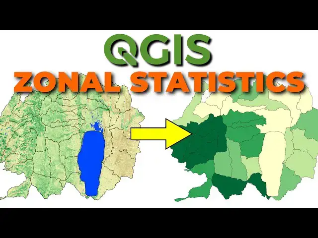
Summarize information from rasters based on polygons with the Zonal Statistics tool in QGIS. This tutorial will demonstrate how to summarize NDVI values for watersheds. This same method can be used to summarize any raster values for any polygon features.
Sentinel-2 Tutorials: https://www.youtube.com/playlist?list=PLoaxBPcx2tRDNJlI8KXkVMl0PO-JCbEqM
Check out my website for more: https://opensourceoptions.com
Show More Show Less View Video Transcript
0:00
Welcome to open source options. Um today
0:04
we're going to discuss how we can take
0:06
raster data and map it to vector data
0:09
using a process called zonal statistics
0:11
so that we can display um summaries of
0:14
our raster data for uh our vector units.
0:19
So let's jump into that. We're going to
0:20
jump into it using some NDVI data from
0:22
Sentinel 2. If you're not sure how to
0:25
calculate NDVI or how to get Sentinel 2
0:28
data, I have videos on that. They'll be
0:30
linked in the description. So, go check
0:33
those out. Um, one more thing before we
0:35
get started. Uh, I have some courses.
0:38
They're going to be some free courses
0:39
coming online at opensource options.com.
0:42
They're not ready yet, but they're going
0:44
to be there. So, you might want to go
0:45
check that out. Uh, by the time you
0:48
watch this video, they could be
0:49
available. Let's jump in to today's
0:52
task. So you'll notice this raster in
0:55
the background. This colored raster with
0:56
the blues and the yellows, browns and
0:59
greens is normalized difference
1:01
vegetation index. It basically shows us
1:03
where green vegetation is. Uh these
1:06
black boundaries are watersheds 12digit
1:10
hydraologic unit codes which is how we
1:12
define some wersheds for smaller
1:14
watersheds that we define in the United
1:17
States.
1:18
What I want to do is I want to take the
1:21
average NDVI value across each of these
1:25
watersheds and map that so I can see
1:27
through time how the vegetation
1:30
greenness is changing across the whole
1:32
wershed. So here I have NDVI for two
1:35
dates. Uh this one's in June the 2024.
1:40
This one is September of 2024. You'll
1:43
notice in the June when we have some
1:45
artifacts in here and these are going to
1:46
be from clouds. Okay, I didn't remove
1:49
the clouds for this example. You'll want
1:50
to make sure you're not you're masking
1:52
out clouds if you do this for a real
1:54
analysis. But here we're not going to
1:57
worry about that. We're just
1:58
demonstrating the concept. So what I
2:00
want to do is calculate the average NDVI
2:04
value in each of these watersheds for
2:06
June and for September. So I can
2:09
visualize it as a function of watershed
2:11
instead of continuously. It's very easy
2:14
to do. We're going to come down here uh
2:16
to this search. I'm going to search for
2:18
zonal
2:19
statistics. Um so if we do
2:22
zonal, we can find this zonal statistics
2:26
here. And we can double click on
2:30
that. All right. If you're not familiar
2:32
with this, you can also go to your
2:34
processing toolbox, which is this button
2:36
up here on the toolbar. This is on the
2:40
Let's close this out so I can see what
2:42
this
2:43
is. Not going to the toolbar. The
2:46
attributes toolbar. We can
2:48
go to the tool box and we can search
2:52
here for
2:55
zonal statistics. We're going to get
2:58
this one here.
3:00
Now, we want to have an input layer.
3:03
It's going to be our vector data here.
3:06
It's my uh huck 12
3:09
watersheds. A raster layer. Let's start
3:12
with June. Um a raster bend. We only
3:15
have one band. So, we're going to get
3:17
that there. And then we can put a column
3:19
prefix on here.
3:24
um which will
3:27
uh be added to a column in our SV table
3:32
and then the statistics to calculate.
3:35
Here we are only going to calculate the
3:37
mean. We you can look and see what all
3:39
these are but this is going to be the
3:41
count of pixels. It's going to be the
3:42
sum of pixel values, the median value,
3:45
uh standard deviation, min, max, range,
3:47
minority, majority, variety, variance.
3:49
So we have a whole lot of different
3:50
things. We only want the mean. You can
3:53
select multiple of these and they'll
3:55
just get added into the attribute name.
3:57
So let's select okay here
4:01
and create temporary
4:04
layer. Let's um we can save this into a
4:08
geo package uh which will make it easier
4:12
or we can append to a layer which is
4:13
what we want to do. So, if we append
4:16
this to a layer, we can come down. Um,
4:20
I'm going to find where this is. Believe
4:23
it's in downloads. And I think I saved
4:27
it in this folder here. So, I'm going to
4:29
just select this
4:30
layer, which is here. And I can add this
4:33
right into my wersheds. So, let's double
4:36
click
4:38
that. Okay. Let's go back. So, it should
4:43
get appended to this layer. And let's
4:45
click
4:49
run. Okay. And so, it's not supported,
4:51
which may happen. Um, we can do this
4:54
again. We'll just
4:57
um save to a geo package. I'll save it
5:01
to the same go package here, which is my
5:04
Huck 12
5:06
selection. And it's going to ask for
5:08
table name. And we'll call this huck 12
5:12
ndvi
5:14
June. We will say
5:17
okay. And we will run
5:20
this. All right. And let's see how this
5:23
finishes. It should finish pretty
5:24
quickly
5:25
[Music]
5:26
here. Okay. So we have that now. Now
5:29
let's go in and look at our attribute
5:31
table. So let's open this
5:34
up. Here we go. We have all the original
5:38
fields. But if I come to the end here,
5:41
we now have NDVI June mean. So we have
5:45
the mean NDVI for every one of those
5:47
watersheds in June. Now let's go and
5:50
let's run this for September. So let's
5:52
run zonal statistics again. Our input
5:55
this time is going to be NDVI June so
5:57
that we can append the September values
6:00
under the end of it. We're going to get
6:01
our September raster. We're going to
6:04
name this
6:05
NDVI September with the underscore after
6:09
it. We're going to calculate just the
6:11
mean. Okay. We're going to save this to
6:17
a geo package. We're going to save it to
6:19
this one. Save. We're going to call this
6:23
hawk 12
6:26
NDVI. We'll call all. So, we'll have all
6:29
the layers. So, we'll say okay. And now
6:33
let's run
6:36
this. Okay. And once again, this take
6:38
just a minute to
6:43
run. Okay. And now we can close this.
6:46
And let's remove our June layer. We
6:48
don't need this anymore. We could delete
6:50
it. We could have saved as a temporary
6:52
layer. There's many ways to deal with
6:53
that. And we can turn that one off. And
6:56
let's open the attribute table. And if
6:59
we come to the end, we have our June
7:02
average NDVI and our September average
7:05
NDVI. And we can see those values are
7:07
indeed different from one another. Now
7:10
we can go in and we can start to
7:12
visualize these differently. So if we
7:14
come here and we go to layer styling and
7:18
we change our single symbol to graduated
7:22
symbols and we change our value to NDVI
7:27
June
7:29
mean and we change our color ramp to
7:35
um let's go view all color
7:39
ramps. Let's
7:44
do we can do brown to blue
7:47
green. Let's try to do
7:51
uh let's do yellow to green. It'll
7:55
probably be the easiest. We can select
7:58
the number of classes and our
7:59
classification method. Um we can do our
8:04
equal
8:05
interval and we can classify it like
8:08
that. Okay, we can also change this to
8:12
like equal count, quantile and we can
8:15
get these various methods for displaying
8:20
the greenness here. Okay, so we get
8:22
different values of cleanness. Now we
8:24
can come in and we can change this to
8:27
[Music]
8:29
September and we can classify
8:33
it and we can see how that changes. So
8:36
using these, we can get an idea of how
8:38
this might change between June and
8:41
September. So let's go ahead and change
8:43
this back to
8:46
June and classify. So let's take a look
8:48
here. We can kind of see where the low
8:50
values are or where the high values are.
8:52
And now let's go
8:57
classify. And we can see now that some
8:59
of those have shifted that June
9:01
generally was greener than September
9:04
was. Okay. Okay, so that's how you can
9:06
easily calculate those statistics for a
9:09
layer and how you can map your raster
9:13
data to vector units. Again, hope you
9:16
found this useful. Go check out the
9:18
courses at opensource
9:20
options.com. I think you'll find them
9:23
useful and enjoy your day.