Up next in 10

It is no longer necessary to perform multiple calculations on Landsat collection 2 level 1 data to calculate surface temperature. With the new Landsat collection 2 level 2 data, it just takes one calculation to have a usable surface temperature layer. This tutorial demonstrates how to download Landsat surface temperature data, convert the Landsat digital number values into actual temperature values, and display the temperature raster in QGIS.
Check out my website for more: https://opensourceoptions.com
How to download Landsat images:
How to visualize satellite images:
How to clip satellite images:
Show More Show Less View Video Transcript
0:01
Welcome to open source options. This
0:03
tutorial will show you how to calculate
0:06
LAN surface temperature from LANCSAT 9
0:09
data. Now this workflow is much simpler
0:12
than it used to be. We can now use
0:15
collection to level two data where we
0:17
just have to convert from dig digital
0:19
number instead of working from the
0:21
collection to level one data which
0:24
required additional calculations to get
0:26
to surface temperature. So it's going to
0:28
be easy. Let's go through and show you
0:30
how it's done. The first thing to do is
0:32
to find a location of interest. I'm
0:34
going to zoom in on an area where we
0:36
should see some good definition in land
0:39
surface temperatures. We have a valley
0:41
over here. If we can find some water in
0:44
there, um that will give us
0:47
uh Oh, good. That will give us a good
0:49
definition between the mountains, the
0:51
valleys, and the water. We have forested
0:53
and unforested areas. Let's go here and
0:56
give this a try. I'm going to click use
0:59
map to select these coordinates to
1:00
search this location. Oh, by the way,
1:03
I'm on earthexplorer.usgs.gov
1:06
to download the LANCAT data. I have a
1:08
full video tutorial on how to do this if
1:10
you're unfamiliar with it. Now, I'm
1:12
going to enter some search dates. So,
1:15
we'll go from about July 21st uh until
1:19
August 11th. And then we'll go over to
1:23
our search results.
1:28
And I should note that on my data sets
1:31
here uh I have LANCAT collection 2 level
1:34
two selected and the LANCAT 8 to9 OI
1:38
tiers data set. Now if we go to our
1:41
results here you can see we have several
1:43
images. Let's go ahead and see what
1:46
these look like in the overlay. So, if I
1:52
uh show the browse overlay, it will show
1:55
me the image.
1:58
Okay, that's not quite the area I was
2:00
looking for. Let's try this one here.
2:04
That's the one I want. That's
2:06
overlapping down further south. Let's
2:08
give that one a try. I'm going to click
2:11
on
2:12
the download options here.
2:16
And then I'm going to click on the
2:17
product options here. And it gives me
2:19
the option to download this entire
2:22
product bundle.
2:26
So I'm going to click that. This will
2:28
take just a minute to download. You can
2:30
see I already have mine downloaded here.
2:32
I downloaded this in preparation. So I'm
2:35
going to click cancel. You download and
2:38
we'll just start working with the data I
2:40
already have. So now I'm going to go
2:42
into QGIS. I'm going to go into my
2:45
browser and I'm going to go find that
2:48
file I downloaded. For me, I have it in
2:50
this LANCAT L2 folder
2:54
and it is this image here that starts
2:58
with the 038033.
3:01
Going to open that image up and I'm
3:03
going to come down and do a couple of
3:05
things. So, first I'm going to add in
3:08
band 10. Notice how it says ST in front
3:11
of band 10. that is the surface
3:13
temperature. Then I'm going to come down
3:15
and grab bands 1 through 7 and add those
3:19
in. And we're going to create a virtual
3:21
raster with these uh just to
3:25
so we can visualize everything. So let's
3:28
go ahead and go to raster miscellaneous
3:32
build virtual raster. Select the inputs.
3:35
I'm going to select one through seven.
3:37
Click select all. Remove band 10. Say
3:41
okay. Place each input file into a
3:44
separate band. I'll save this to a
3:46
temporary file for now. We're not going
3:48
to need this later. And click run.
3:52
And now I'm going to say close.
3:55
Now the next thing I'm going to do is
3:58
I'm going to limit this to just a small
4:00
area. I don't need to calculate this for
4:02
everywhere. Um but I do want to
4:04
calculate it for a small area. And I'm
4:06
going to use my virtual raster to find
4:08
that area that's going to work best. I
4:10
want to find an area that's going to
4:12
have some land surface temperature
4:13
variation to make it easier to see these
4:16
changes. So, let's uh change this to
4:21
bands 432 so we get a true color image.
4:25
There's our true color. And now we can
4:27
zoom in to see if we can find an area
4:29
where there should be some variation
4:32
in our temperatures. This looks like a
4:36
good spot here. We can see we have a
4:37
reservoir or a lake up here. We have
4:39
some higher mountains, some lower
4:41
valleys, and some more water over in
4:43
this area. So, if we focus on this
4:45
location, we should see some temperature
4:47
variation. I'm now going to clip this
4:50
image down to that area so we're not
4:53
calculating on such a large area. So to
4:56
do that, let's go to raster. Let's go to
4:59
extraction clip raster by extent. Now I
5:03
have a full video on how to do this also
5:05
if you're interested in that. I'm going
5:06
to work work through it quickly here. So
5:09
we can drop this down. I'm going to calc
5:12
or draw on the map canvas. Excuse me.
5:16
I'm just going to draw a rectangle so
5:18
that it encompasses some of these areas
5:21
here.
5:22
something like
5:25
this.
5:27
That gives me the extent. And now I can
5:29
come down. We will save this as a
5:32
temporary layer. And I want to make sure
5:34
I have the correct clipping layer
5:35
selected. I want to clip um layer band
5:40
10 here.
5:43
And let's click well let's let's say
5:48
well let's click run. There we go. Let's
5:49
click run. Now we can close this. So you
5:52
can see we have band 10 clipped to this
5:54
location.
5:56
Now the next step, the next thing we
5:58
need to do is we need to find our
6:00
conversion to convert band 10 from its
6:04
digital number into an actual
6:08
temperature which we can do as degrees
6:10
Kelvin, degrees Celsius or degrees
6:11
Fahrenheit. Let me show you how to do
6:13
that. So we can come over to the
6:15
internet here and let's do LANCAT level
6:18
two temperature. if we search for that
6:21
and we can come to the USGS
6:22
documentation here and this will give us
6:25
some additional insight in how to do
6:27
this. So here's the documentation for
6:30
this band. Notice here it gives us the
6:33
scaling factor. So to interpret this we
6:35
need the digital number which is the
6:36
value in our raster band multiplied by
6:40
this constant with this added constant
6:42
here. This is really easy to do. So
6:45
let's uh go back to QGIS and perform a
6:48
raster calculation to get this done.
6:52
So now we'll go to raster
6:55
raster calculator.
6:57
Pull that over here. We want our clipped
6:59
band 10 to start out with. So I'm going
7:02
to close this up here. Inside of
7:04
parentheses, we're going to multiply it
7:06
by a constant and we're going to add 149
7:10
to it. So let's go grab that constant so
7:12
we can make sure we get this correct.
7:15
and it's going to be here. So, it's
7:18
0.00341802.
7:23
Probably do this in two tries, but we'll
7:25
get it. 034
7:34
and then let's go get the rest of that
7:35
number here. And it is 1802.
7:42
Now when we multiply this, this will
7:44
give us our value in Kelvin.
7:49
So let's save this.
7:52
And
7:54
we already have a test file in here, but
7:56
we'll call it our surface temperature in
7:58
Kelvin. So we can save that.
8:03
We'll overwrite it. I'm going to click
8:05
okay to run this.
8:08
You can see it's completed. So our
8:10
values range from 295 Kelvin to 333
8:14
Kelvin. We can change this symbology
8:20
so that we have lower values occurring
8:22
in blue and higher values in red. And
8:25
you can see there that we easily uh can
8:28
see the low temperatures crew over water
8:30
as they should and in the mountains as
8:32
they should. And our higher temperatures
8:35
if we switch back to our virtual color
8:38
raster these high values are occurring
8:42
uh on these slopes without vegetation.
8:45
We can also see these agricultural
8:47
fields have low values. Now, let me show
8:50
you how we can convert this into degrees
8:52
Celsius or degrees Fahrenheit, which is
8:55
something you might be more uh familiar
8:58
with. So, to do this, we just need to do
9:01
another raster calculator
9:04
and we're just going to take our degrees
9:06
Kelvin
9:10
and we'll go find the correct conversion
9:12
so that I get it right. But I believe if
9:14
we're going to Fahrenheit,
9:17
we'll do minus
9:19
273.15
9:21
Kelvin
9:23
multiply
9:25
by 9/5s
9:27
and add 32. So this should give it to us
9:30
in Fahrenheit. If we wanted it in
9:32
Celsius, we should just have to subtract
9:35
this 273.15.
9:37
But let's just check that conversion on
9:39
the internet real quick. So let's go
9:41
convert Kelvin to Fahrenheit. And you
9:45
can see here we have our Kelvin minus
9:48
273.15
9:49
that exact same equation. If we change
9:52
this to Celsius,
9:56
then it is indeed we just subtract
9:59
273.15.
10:01
So with those we can run this
10:03
calculation. Let's save this to a file.
10:07
And you'll see that I've already have
10:09
this one here. We'll save it to
10:10
Fahrenheit. So, let's save that. Let's
10:14
replace it. Let's say okay. That's going
10:18
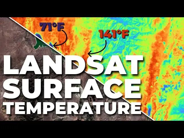
to run. And we can now change this to
10:20
single band pseudo color with that same
10:23
symbology. You can see that our values
10:25
range from 71° F to 141° F. And those
10:31
seem to fall in an acceptable range for
10:33
Fahrenheit values. If you're in a
10:35
country where Celsius is your standard
10:37
temperature units, uh then you can go do
10:40
this in Celsius. But that's how you can
10:43
very easily calculate surface
10:45
temperature in QGIS from Lancet data. I
10:49
hope you found this useful. If you like
10:51
this tutorial, check out my channel for
10:53
other tutorials and check out opensource
10:55
options.com where I'm going to be having
10:57
some free online courses for GIS and
11:00
remote sensing. I've started the first
11:02
one already. Once that's done, there are
11:04
more coming. Thanks for watching.