Vectorize Moving Window Grid Operations on NumPy Arrays

There’s a good chance you’ve done something today that used a sliding window (also known as a moving window) and you didn’t even know it. Have you done any photo editing? Many editing algorithms are based on moving windows. Do you do terrain analysis in GIS? Most topographic raster metrics (slope, aspect, hillshade, etc.) are based on sliding windows. Anytime you do analysis on data formatted as a two-dimensional array there’s a good chance a sliding window will be involved.

Sliding window operations are extremely prevalent and extremely useful. They’re also very easy to implement in Python. Learning how to implement moving windows will take your data analysis and wrangling skills up to a new level.

What is a Sliding Window?

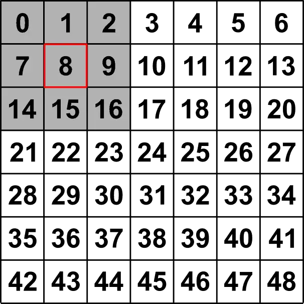
The example below shows a 3×3 (3 by 3) sliding window. The array element outlined in red is the target element. This is the array location the sliding window will calculate a new metric for. For example, in the image below, we could calculate the mean of the 9 elements in the grey window (spoiler alert, the mean is also 8) and assign it to the target element, which is outlined in red. Instead of the mean, you could calculate the minimum value (0), the maximum value (16), or a number of other metrics. This is done for each element in the array.

That’s it. That’s the basics of sliding windows. Of course, things can get much more complicated. Finite difference approaches can be used for temporal and spatial data. Logic can be implemented. Larger window sizes or non-square windows can be used. You get the idea. But at its core, moving window analysis can be summed up as simply as the mean of neighbor elements.

It’s important to note that special accommodations must be made for edge elements because they don’t have 9 neighbors. Because of this many analyses exclude edge elements. For simplicity, we’ll exclude edge elements in this article.

Create a NumPy Array

To implement some simple examples, let’s create the array shown above. To start, import numpy.

import numpy as np

Then use arange to create a 7×7 array with values that range from 1 to 48. Also, create another array filled with no data values that is the same shape and data type as the initial array. In this instance, I’m using -1 as the no-data value. For a complete guide to filling NumPy arrays, you can check out my previous article on the topic.

a = np.arange(49).reshape((7, 7)) 
b = np.full(a.shape, -1.0)

We’ll use these arrays to develop the sliding window examples that follow.

Sliding Window with a Loop

No doubt, you’ve heard that loops in Python are slow and should be avoided where possible. Especially when working with large NumPy arrays. What you’ve heard is quite correct. Nevertheless, we’ll first go through an example that uses a loop because it’s an easy way to conceptualize what is happening in a moving window operation. After you’ve grasped the concept with the loop example, we’ll move on to a more efficient, vectorized approach.

To implement a moving window, simply loop over all of the interior array elements, identify the values for all neighbor elements, and use those values in your specific calculation.

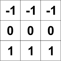
Neighbor values are easily identified with row and column offsets. Offsets for a 3×3 window are given below.

Python Code for a NumPy Moving Window in a Loop

We can implement a moving window in three lines of code. This example calculates the mean within the sliding window. First, loop over interior rows of the array. Second, loop over interior columns of the array. Third, calculate the mean within the sliding window and assign the value to the corresponding array element in the output array.

for i in range(1, a.shape[0]-1):
    for j in range(1, a.shape[1]-1):
        b[i, j] = (a[i-1, j-1] + a[i-1, j] + a[i-1, j+1] + \
                   a[i, j-1] + a[i, j] + a[i, j+1] + a[i+1, j-1] + \
                   a[i+1, j] + a[i+1, j+1]) / 9.0

Sliding Window Loop Result

You’ll notice the result has the same values as the input array, but the exterior elements are assigned no data values because they do not contain 9 neighbor elements.

[[-1. -1. -1. -1. -1. -1. -1.]
 [-1.  8.  9. 10. 11. 12. -1.]
 [-1. 15. 16. 17. 18. 19. -1.]
 [-1. 22. 23. 24. 25. 26. -1.]
 [-1. 29. 30. 31. 32. 33. -1.]
 [-1. 36. 37. 38. 39. 40. -1.]
 [-1. -1. -1. -1. -1. -1. -1.]]

Vectorized Sliding Window

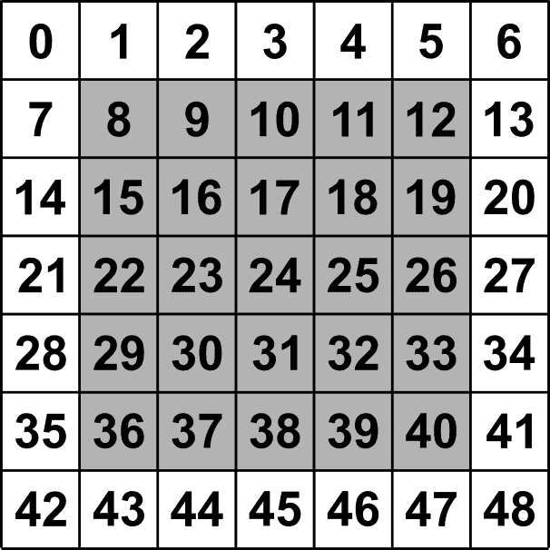
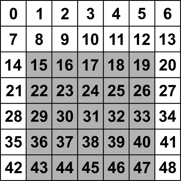
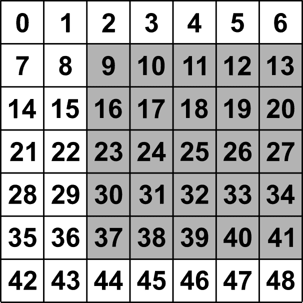
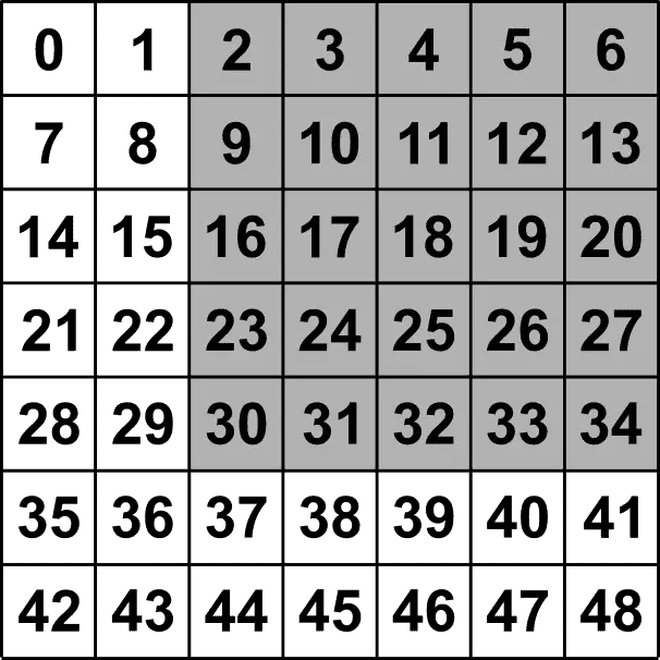
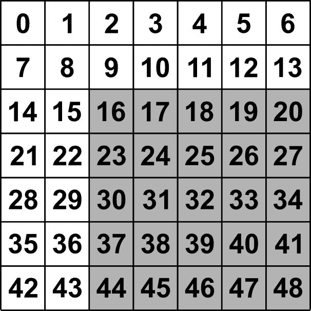
As you know, loops over arrays in Python are usually computationally inefficient. Efficiency can be increased by vectorizing operations that would normally be done in a loop. Moving window vectorization can be accomplished by offsetting all of an array’s interior elements simultaneously.

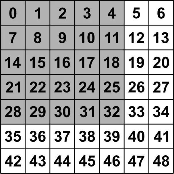
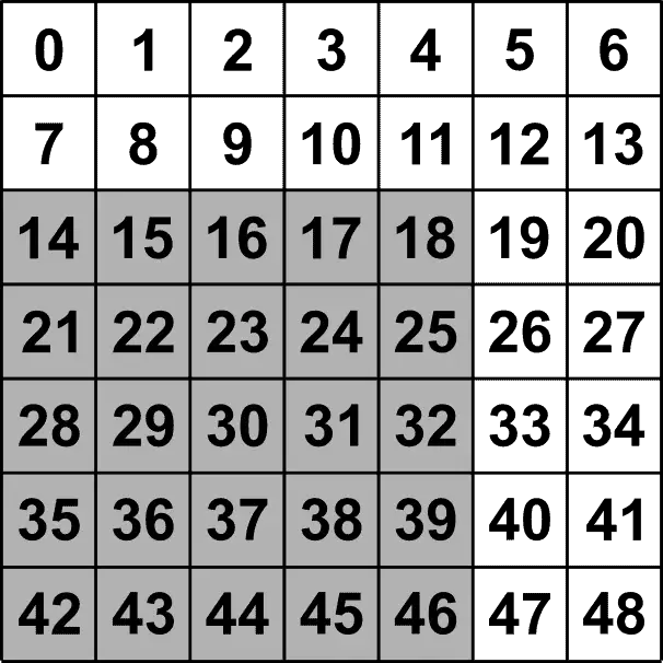
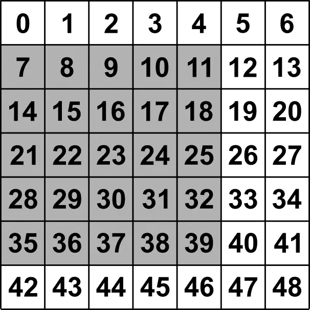
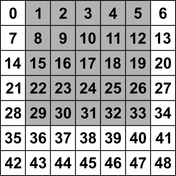
This is demonstrated in the images below. Each image is captioned with the corresponding indices. You’ll notice the first image indexes all of the interior elements, and corresponding images index offsets to each neighbor.

Python Code for a Vectorized Moving Window on a Numpy Array

With the offsets described above, we can now easily implement a sliding window in one line of code. Simply set all the interior elements of the output array equal to your function that calculates the desired output based on the neighbor elements.

b[1:-1, 1:-1] = (a[1:-1, 1:-1] + a[:-2, 1:-1] + a[2:, 1:-1] + a[1:-1, :-2] + a[1:-1, 2:] + a[2:, 2:] + a[:-2, :-2] + a[2:, :-2] + a[:-2, 2:]) / 9.0

Vectorized Sliding Window Result

As you can see, this gives the same result as the loop.

[[-1. -1. -1. -1. -1. -1. -1.]
 [-1.  8.  9. 10. 11. 12. -1.]
 [-1. 15. 16. 17. 18. 19. -1.]
 [-1. 22. 23. 24. 25. 26. -1.]
 [-1. 29. 30. 31. 32. 33. -1.]
 [-1. 36. 37. 38. 39. 40. -1.]
 [-1. -1. -1. -1. -1. -1. -1.]]

Speed Comparison

The two methods demonstrated above produce the same result, but which one is more efficient? I calculated the speed of each method for arrays ranging from 5 rows and columns to 100. Each method was tested 100 times for each array. The mean time for each method is plotted below.

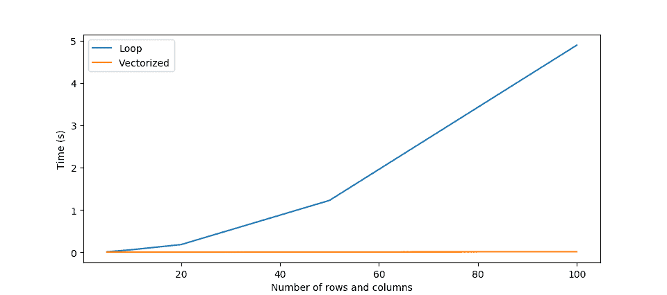
It’s quite obvious that the vectorized approach is much more efficient. The loop’s efficiency decreases exponentially as array size increases. Also, note that an array with 10,000 elements (100 rows and 100 columns) is quite small. For example, full-resolution images from smartphone cameras are going to have greater than 2,000 rows and columns.

Conclusion

Moving window calculations are extremely common in many data analysis workflows. These calculations are very useful and very easy to implement. However, implementing sliding window operations with loops is extremely inefficient. A vectorized moving window implementation is not only more efficient but also uses fewer lines of code. Once you get the hang of the vectorized approach for implementing sliding windows you can easily and efficiently increase your workflow speed.