Interactive Split-Screen Map with Python
Visualizing raster data is important for assessing the results of analysis and models. One of the best ways to visualize raster data is to plot it on a map where you can interact with the raster data an other relevant layers.
When performing analysis in Python, it can be difficult to create an interactive map. This often means that data layers must be exported from a Python script or program and opened in other GIS software (such as ArcGIS or QGIS) to be viewed.
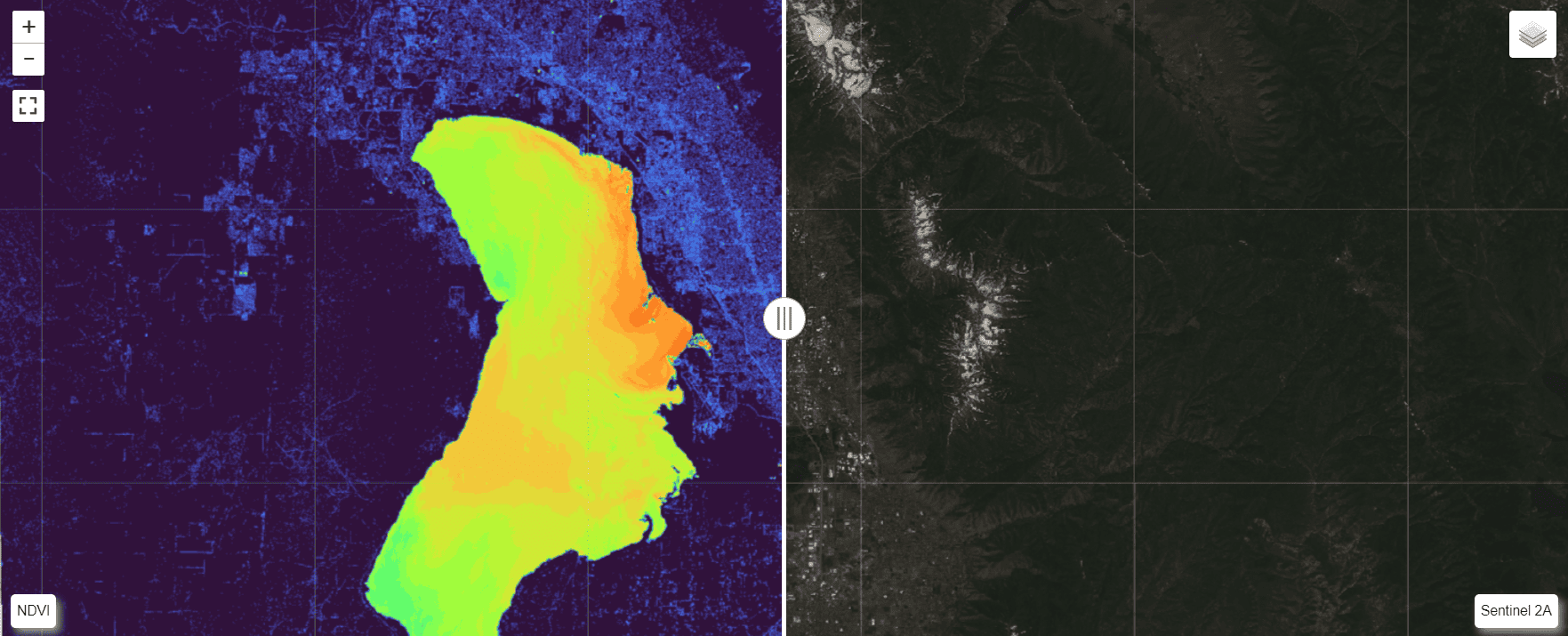
Leafmap is a Python package to create interactive maps directly in Jupyter notebooks. It allows adding raster layers that are saved to disk and xarray data. Leafmap even supports a split-screen swipe view to easily compare different data layers.
Follow along with this tutorial to use leafmap to create an interactive Python map with a split-screen, swipe view.
Data
For this tutorial we’ll use an image from Sentinel 2A which we can dispaly in true and false color. We’ll also use the Sentinel 2A data to calculate NDVI.
You’ll need to have Sentinel 2A data downloaded to your machine to follow along.
Sentinel images can be freely downloaded from a variety of sources. I prefer to go directly to the source, the Copernicus Browser.
Environment and packages
You’ll need a few packages to perform the visualizations and analyses in this tutorial. I recommend using a minconda distribution and using conda and mamba to install the packages.
The packages to install and import are listed in the code block below. You can follow along with me as I set up the environment and packages in the video at the end of this article.
from osgeo import gdal
import leafmap
import xarray as xr
import rioxarray
C:\Users\Konrad\miniconda3\envs\split\lib\site-packages\pandas\core\computation\expressions.py:21: UserWarning: Pandas requires version '2.8.4' or newer of 'numexpr' (version '2.7.3' currently installed).
  from pandas.core.computation.check import NUMEXPR_INSTALLED
Create a virtual raster
Sentinel collects data for 13 different bands. Each band contains reflectance data for a different wavelength of light. These data are stored in individual raster files.
To display the sentinel images, we want to have them included in the same file. We’ll do this using the virtual raster format. The virtual format is basically a metadata file that takes information from multiple rasters so they can be combined without actually processing the underlying data.
We’ll create a virtual raster using just bands 2-5 (blue, green, red, near infrared).
# Create a virtual raster from Sentinel 2a image

# path to a Sentinel 2A image
sen2a_base = r"path\to\sentinel\image\S2A_MSIL1C_20230626T180921_N0509_R084_T12TVK_20230626T215620.SAFE\S2A_MSIL1C_20230626T180921_N0509_R084_T12TVK_20230626T215620.SAFE\GRANULE\L1C_T12TVK_A041837_20230626T181453\IMG_DATA\T12TVK_20230626T180921_B{0}.jp2"
sen2a_fns = []
vrt_fn = "../data/my.vrt"

for band_num in range(2, 6):
    sen2a_fns.append(sen2a_base.format(str(band_num).zfill(2)))

sen2_vrt = gdal.BuildVRT(vrt_fn, sen2a_fns, separate=True)
sen2_vrt = None
Once the VRT is built. Set the variable to None so the file writes to disk.
Calculate NDVI
Next calculate NDVI as an xarray data array. We can display this data type without needing to write a file to disk.
Open the VRT as an xarray using rioxarray.
Then apply the NDVI equation with bands 3 (Red) and 4 (NIR), as shown below.
sen2_xr = rioxarray.open_rasterio(vrt_fn)
ndvi = (sen2_xr.sel(band=4) - sen2_xr.sel(band=3)) / (sen2_xr.sel(band=4) + sen2_xr.sel(band=3))
Now create the map with leafmap.
Start by creating a leafmap.Map object, then apply the split_map function. Now specify the left layer (ndvi), right layer (enter the file name for the VRT), left label, and right label. The left and right args are dictionaries of arguments that correspond to leafmap.add_raster_layer.
For the sentinel image, specify the band combination to apply. A combination of [3, 2, 1] will give true color and [4, 3, 2] will give color infrared.
Run the code and your map will be ready. It may take a few minutes for the map and data to load.
m = leafmap.Map()
m.split_map(
    ndvi,
    vrt_fn,
    left_label="NDVI",
    right_label="Sentinel 2A",
    left_args={
        "layer_name": "NDVI",
        "colormap": "turbo"
    },
    right_args={
        "layer_name": "Sentinel 2A",
        "bands": [4, 3, 2]
    }
)
m
Map(center=[20, 0], controls=(ZoomControl(options=['position', 'zoom_in_text', 'zoom_in_title', 'zoom_out_text…
Video
Conclusion
Leafmap provides an excellent Python package for geospatial data visualization. When paired with xarrary, it also provides a nice way to view analysis results without the need to write data to disk and open it in a different application.
The split map with swiping provides a nice touch for data visualization and comparisons.


