How to Create a DEM (or Raster) from a Lidar Point Cloud
Lidar data are 3D point clouds that can describe Earth’s surface in great detail. However, lidar point clouds present some challenges because of how much data they contain. One fundamental challenge with lidar data is how to effectively extract the points that represent the Earth’s surface (not vegetation, building, or other objects) and create a DEM (or DTM).
This tutorial will demonstrate how to use PDAL, a powerful, open-source library to create a bare-earth DEM from a lidar point cloud.
Apply a Ground Filter to the Point Cloud
The first step to creating a DEM (or DTM) from a lidar point cloud is to identify the lidar returns that represent the ground and not vegetation or other surfaces. This is referred to as ground filtering. We can perform a ground filter by creating a PDAL pipeline, which is a list of commands that are executed in sequence. PDAL pipelines are defined as JSON files. The pipeline below performs ground filtering on a lidar point cloud. Let’s go through it and explain what’s going on.
{
  "pipeline":[
    {
      "type":"filters.reprojection",
      "out_srs":"EPSG:26911"
    },
    {
      "type":"filters.assign",
      "assignment":"Classification[:]=0"
    },
    {
      "type":"filters.elm"
    },
    {
      "type":"filters.outlier"
    },
    {
      "type":"filters.smrf",
      "ignore":"Classification[7:7]",
      "slope":0.2,
      "window":16,
      "threshold":0.45,
      "scalar":1.2
    },
    {
      "type":"filters.range",
      "limits":"Classification[2:2]"
    }
  ]
}
The PDAL Pipeline
PDAL uses pipelines to create workflows by linking commands. Pipelines link together readers, filters, and writers.
The JSON file specified above is a PDAL pipeline that uses a list of filters to create a ground filtered point cloud, which is a point cloud that only contains points representing the ground surface and not vegetation. I’ll go through the pipeline components and JSON structure below.
Let’s start with "pipeline". This is an array of objects. Each object is grouped with curly braces {} and specifies a PDAL command and its associated parameters.
For each PDAL command, "type" specifies the command, and all other keys/variables specify the command’s arguments.
Reproject the Point Cloud
The first object specifies the filters.reprojection command. This reprojects the input point cloud. Reprojection of point clouds is often necessary to ensure the points are referenced to a linear coordinate system. In this case, the input point cloud will be reprojected to NAD83 UTM Zone 11N.
Reclassify all Points to 0
filters.assign gives all the points in the point cloud a classification value of 0. Lidar specification defines a classification of 0 as points that are created but never classified. This command effectively resets the classification of all points.
Remove Low-Noise Points
The extended local minimum (ELM) algorithm identifies points that have low noise and are likely not suitable for analysis. The PDAL filter filters.elm implements the ELM algorithm. This command will identify low-noise points with ELM and classify them with a value of 7, which represents noise points in accordance with lidar specs.
Remove Outliers
Next, we’ll apply an outlier filter to identify points that don’t seem to fit with points around them. Points identified as outliers are given a classification of 7. You can read more about outlier identification in the PDAL documentation.
The SMRF Ground Segmentation Algorithm
Now it’s time for the meat of the operation. Until this point, we’ve just been setting up the point cloud and removing noise (i.e. points that potentially contain errors). The ground segmentation algorithm is what will actually give us a point cloud of ground-only points.
Here we use the Simple Morphological Filter (or SMRF) for ground segmentation. This is a PDAL implemented algorithm based on this publication.
Basically, SMRF has been optimized to identify ground points that will create a detailed DEM. If you want more detail than that you can dig into the details of the publication linked above.
Here is a simple description of the SMRF parameters.
"ignore"tells SMRF not to use points with classification of 7 in the segmentation."slope"is a slope threshold used to identify points that are associated with objects (trees, building, etc) and not the ground"window"specifies the maximum distance/radius for the SMRF window to be applied within the point cloud"treshold"is an elevation threshold used to identify objects"scalar"is an elevation scaling factor.
For more information follow the links to the PDAL documentation and the SMRF publication.
The SMRF filter will identify ground points according to the input parameters and classify them with a value of 2.
Extact Ground Points
Now that we have identified ground points with SMRF we want to extract only these points so they can be saved to a separate point cloud. This is done with a PDAL range filter(filters.range).
Specify the "limits" variable to select all points with a classification of 2 as shown in the JSON file.
Run the PDAL Pipeline
Once you have the JSON file constructed, run it using pdal translate. You can use the command syntax below where input.laz is the original (or input) point cloud and ground.laz is the result point cloud (or ground filtered point cloud). The --json argument specifies the path to the JSON file that contains code for your pipeline. Note: this command can take several minutes to run depending on your computer hardware and the size of your point cloud.
pdal translate input.laz ground.laz --json pipeline.json
Write the Gound-Filtered Point Cloud to a Raster
Now that we’ve created a ground-filtered point cloud that is optimized for a DEM it is time to create the DEM. This is done by using the ground-filtered point cloud to create a raster.
Once again we will use a PDAL pipeline. This pipeline will only contain a single command.
After specifying the "pipeline" array we give the path to the input point cloud, which is the ground.laz (output point cloud) from the pipeline above.
Now give the filename of the output dem ("filename"), the GDAL driver to use to create that file ("gdaldriver"; see a list of GDAL drivers here), the statistics to calculate for the new raster ("output_type"), and the resolution of the output raster in units corresponding to your specific CRS ("resolution"; here it is 1 meter).
We’ll use a PDAL writer filter (writers.gdal) to create the output file.
{
    "pipeline": [
		"path/to/ground.laz",
        {
            "filename":"dem.tif",
            "gdaldriver":"GTiff",
            "output_type":"all",
            "resolution":"1.0",
            "type": "writers.gdal"
        }
    ]
}
Once your pipeline JSON file is ready, run it with pdal pipeline and pass the name of the pipeline JSON file. Note: the output will be created in the current working directory of your terminal.
pdal pipeline path/to/gdalwriter.json
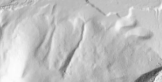
Once the command has finished executing you will have generated a bare-earth DEM from the point cloud.
Conclusion
Initially, it requires some work to create the ground-filtered point cloud and DEM. But now you have a workflow that can be used over and over again. All you have to do is change file names and maybe adjust some parameters for specific instances. Happy processing.
